2.1. Refraction: lens#
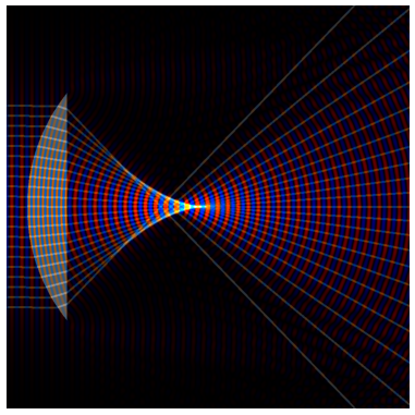
The main role of this simulation is to look at the the phase imprinting property of a lens or lens refraction see Sec. 2.15-2.18 of Opticsf2f. We shall add rays which follow the law of Ibn Sahl, Sec. 2.7. This allows us to compare ray optics and wave optics, at least for the case of a small lens. For a simpler case of refraction, see also an example using a prism, PrismRefraction.ipynb
The simulation makes use of some topics covered in later Chapters: For example, we shall propagate the electric field using the hedgehog equation, Sec. 6.4. Also the input field is a gaussian beam, see Sec. 11.3. However, we do not necessarily need to understanding exactly how the simulation is construction in order to understanding the basis properties of lens. Also important to note is that the propagation code is paraxial so we can expect significant errors when the angle between the propagation direction and the surface normal is greater than about 30 degrees.
First we explore the physics using an interactive figure.
Below we shall include the code that produces the images.
There are many cools results in this simulation. A few of my favourites are:
The rays do not all converge on a single point due to spherical aberrations. The rays closer to the optical axis converge at the focus.
Looking at the field, we can see how the waves compress inside the lens.
And how the lens imprints wavefront curvature.
Note how the focus of the gaussian beam (beam waist) is ‘upstream’ of the ray focus.
Note how the wavefronts are curved in the focal plane (indicated by the ray focus).
Note how the field and intensity distributions are asymmetric upstream and downstream of the focus.
At least three of these, we miss if we only plot intensity!
Next, we look at the code that generates the images above. You can run the code in your browser. Note that the first two cells that import python packages may take up to 10 s each depending on your platform.
The Jupyter Notebook is LensRefraction.ipynb see
import time
start_time = time.time()
import matplotlib.pyplot as plt
import numpy as np
from numpy.fft import fft, ifft, fftshift
print("--- %s seconds ---" % (time.time() - start_time))
--- 0.5348672866821289 seconds ---
First we define some 2D functions. We use GBeam to plot a gaussian beam, Line to draw a ray and Circle to define the convex surface of a lens.
def Line(x,y,x1,y1,x2,y2,a):
    x0 = (x1+x2)/2
    y0 = (y1+y2)/2
    rotation = -np.arctan((x1-x2)/(y1-y2+1e-8))
    b = np.sqrt((x1-x2)**2 + (y1-y2)**2) # length of line
    xa = (x-x0)*np.cos(rotation) + (y-y0)*np.sin(rotation)
    ya = (y-y0)*np.cos(rotation) - (x-x0)*np.sin(rotation)
    return (xa > (-a/2)) & (xa < (a/2)) & (ya > (-b/2)) & (ya < (b/2))

def GBeam(zb,yb,z0,y0,beamsize,angle):
    angle = angle
    za = (zb-z0)*np.cos(angle) + (yb-y0)*np.sin(angle)
    ya = (yb-y0)*np.cos(angle) - (zb-z0)*np.sin(angle)
    zR = np.pi*beamsize**2
    q = za-1.j*zR
    return (-1.j*zR*np.exp(2*np.pi*1.j*(za+ya*ya/(2*q)))/q)

def Circle(x,y,x0,y0,r):
    xa = x-x0
    ya = y-y0
    return (xa*xa + ya*ya < (r*r))
Next we define a grid in units of the wavelength. \(dy\) and \(dz\) are the spatial resolution - \(\lambda/40\) for the values given below. The \(z\) axis will be the propagation direction.
zmin = 0 # z is the horizontal axis so like x in cartesian system
zmax = 40
ymin = -20   # vertical axis coould be x or y, call it y to agree with standard axes
ymax = 20
dz = 0.05
dy = 0.05
zoom = 1
Z, Y = np.mgrid[zmin/zoom:zmax/zoom:dz/zoom,ymin/zoom:ymax/zoom:dy/zoom]
z_pts, y_pts = np.shape(Z)
This is the corresponding (Fourier) \(k\)-space grid to be used in the hedgehog propagation.
kymax=1.0*np.pi/dy
dky=2*kymax/y_pts
ky=np.arange(-kymax,kymax,dky) # fourier axis scaling
ky2=ky*ky
ky2c=ky2.astype('complex') #Notes on complex types http://www.scipy.org/NegativeSquareRoot
k=2.0*np.pi # k=2pi/lambda with lambda_0=1
k2=k*k
kz=np.sqrt(k2-ky2c)
This is the propagation phase the appears in the hedgehog equation.
ph=1.0j*kz*dz
We define region with higher refractive index to produce a plano-convex lens.
Radius = 18.0
Radius2=Radius*Radius
ZPos= zmax/2
YPos= 0
LensBack = 6
Lens = Circle(Z,Y,ZPos,YPos,Radius) * (Z < (LensBack))
Next, a function to draw rays.
def DrawRays(R,G,B,NRays,RaySep,RayWidth,BeamOffset,Index):
    for RayDisp in range (-NRays,NRays+1,1):
        ZR1 = 0
        YR1 = BeamOffset + RayDisp * RaySep
        if np.abs(YR1) < Radius:
            ZR2 = ZPos - np.sqrt(Radius**2 -  YR1**2)
            YR2 = np.sign(YR1)*np.sqrt(Radius**2 - (ZR2-ZPos)**2) # eqn or incomping ray
            R += 0.2 * Line(Z,Y,ZR1,YR1,ZR2,YR2,RayWidth)
            Theta_i = np.arccos(-(ZR2-ZPos)/Radius)
            Theta_t = np.arcsin(np.sin(Theta_i)/Index)
            BAngle2 = np.sign(YR1)*(Theta_t - Theta_i)
            ZR3 = LensBack
            YR3 = (ZR3-ZR2)*np.tan(BAngle2) + YR2
            R += 0.2 * Line(Z,Y,ZR2,YR2,ZR3,YR3,RayWidth)
            BAngle3 = np.arcsin(np.clip(np.sin(BAngle2)*Index,-1.0,1.0))
            ZR4 = zmax
            YR4 = (ZR4-ZR3)*np.tan(BAngle3) + YR3
            R += 0.2 * Line(Z,Y,ZR3,YR3,ZR4,YR4,RayWidth)
        else:
            ZR2 = zmax
            YR2 = YR1
            R += Line(Z,Y,ZR1,YR1,ZR2,YR2,0.1)
    G += R
    B += R
    return R, G, B
These are the parameters your might want to change.
Index = 2.2
BeamSize = 10
Rays = "Rays" # or "No Rays"
E_or_I = "Field" # or "Intensity"
The next cell is the core of the code. The first few lines initialise the grid, then we add the lens and a gaussian beam in the input plane. The hedgehog propagation is in the jj loop. Finally, we add the output, either electric field or intensity, into the RGB channels, and plot.
start_time = time.time()

R = np.zeros((z_pts,y_pts))
G = np.zeros((z_pts,y_pts))
B = np.zeros((z_pts,y_pts))

NR = np.zeros((z_pts,y_pts))
NR += (Index - 1)*Lens
BAngle = 0*np.pi/180
BeamOffset = 0

if (Rays == "Rays"):
    NRays = 10
    RaySep = 1
    RayWidth = 0.2
    R, G, B = DrawRays(R, G, B, NRays, RaySep, RayWidth,0,Index )

E0 = GBeam(Z[0,:],Y[0,:],0,BeamOffset,BeamSize,BAngle)
b = fftshift(fft(E0))
for jj in range (0,z_pts): # propagation
        c = ifft(fftshift(b)) * np.exp(2.0j*np.pi*NR[jj,:]*dz)
        b = fftshift(fft(c)) * np.exp(1.0j*kz*dz)
        if (E_or_I == "Field"):
            R[jj,:] -=  0.5*c.real
            B[jj,:] +=  0.5*c.real
        if (E_or_I == "Intensity"):
            G[jj,:] +=  0.2*(abs(c)*abs(c))**0.5

fig, (ax1) = plt.subplots(1,1,figsize=(8, 8),dpi=60)

R+=0.3*(Index-1)*Lens # add lens to final image
G+=0.3*(Index-1)*Lens
B+=0.3*(Index-1)*Lens

br=1.0
bg=1.0
bb=1.0

R=np.clip(br*R,0.0,1.0)
G=np.clip(bg*G,0.0,1.0)
B=np.clip(bb*B,0.0,1.0)
RGB=np.dstack((np.flipud(R.T), np.flipud(G.T), np.flipud(B.T))) # use transpose to swap image axes, flipud to origin at bottom left

ax1.imshow(RGB)
print("--- %s seconds ---" % (time.time() - start_time))
ax1.set_axis_off()
--- 0.9482014179229736 seconds ---