2.3. Dispersion: prism

This code is the same as PrismRefraction.ipynb except that here we are going to use three colours.

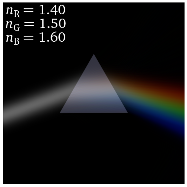
We can set the refractive indices for each colour separately and hence explore dispersion.

The images we create is iconic. Newton’s in his so called experimentum crucis studied prism refraction of sunlight adding a second prism in the red path to show that you cannot split a primary colour. However, the claim Newton made was not actually true as the red light still has a range of wavelengths which diverge after a second prism.

The image is also iconic as a similar image was used as the album cover for Dark Side of the Moon by Pink Floyd in 1973. A good exercise is to see if you think there is a problem with their back cover?

Next, we explore the code that generates the images in the interactive figure above.

The Jupyter Notebook is Disp.ipynb see

opticsf2f/Opticsf2f_CodeBook

CLICK HERE TO ACTIVATE CODE CELLS

import matplotlib.pyplot as plt
import numpy as np
import time
import matplotlib.colors as colors
from numpy.fft import fft, ifft, fftshift

import matplotlib as mpl
mpl.rcParams['font.family'] = 'serif'
mpl.rcParams["text.latex.preamble"]  = r"\usepackage{amsmath} \usepackage{amssymb} \usepackage[bitstream-charter]{mathdesign}"
mpl.rcParams["text.usetex"] = True

This cell defines a few functions. We shall use Triangle for a prism and GBeam for our input light.

def GBeam(zb,yb,z0,y0,beamsize,angle):
    angle = angle
    za = (zb-z0)*np.cos(angle) + (yb-y0)*np.sin(angle)
    ya = (yb-y0)*np.cos(angle) - (zb-z0)*np.sin(angle)
    zR = np.pi*beamsize**2
    q = za-1.j*zR
    return (-1.j*zR*np.exp(2*np.pi*1.j*(za+ya*ya/(2*q)))/q) 

def Triangle(x,y,x0,y0,size,angle):
    return ((-y-y0 + size/(2*np.cos(angle/2))-np.tan(angle)*(x-x0) > (0)) 
            &  (-y-y0 + size/(2*np.cos(angle/2))+np.tan(angle)*(x-x0) > (0)) 
            & (-y-y0 + size/(2*np.cos(angle/2)) < (size*np.cos(angle/2))))

Next we define a grid in units of the wavelength. \(dy\) and \(dz\) are the spatial resolution. \(\lambda/50\) for the values given below.

zmin = 0 # z is the horizontal axis so like x in cartesian system
zmax = 160
ymin = -80   # vertical axis coould be x or y, call it y to agree with standard axes
ymax = 80
dz = 0.1
dy = 0.1
zoom = 1
Z, Y = np.mgrid[zmin/zoom:zmax/zoom:dz/zoom,ymin/zoom:ymax/zoom:dy/zoom]
z_pts, y_pts = np.shape(Z)

This is the \(k\)-space grid.

kymax=1.0*np.pi/dy 
dky=2*kymax/y_pts
ky=np.arange(-kymax,kymax,dky) # fourier axis scaling
ky2=ky*ky
ky2c=ky2.astype('complex') #Notes on complex types http://www.scipy.org/NegativeSquareRoot
k=2.0*np.pi # k=2pi/lambda with lambda_0=1
k2=k*k
kz=np.sqrt(k2-ky2c)

This is the propagation phase the appear in the hedgehog equation.

ph=1.0j*kz*dz

We define triangle that will become our prism

PSize = 60
PAngle = 60*np.pi/180
PCentre = PSize/(2*np.cos(PAngle/2))
PWidth = PSize*np.sin(PAngle/2)
Prism = Triangle(Z,Y,zmax/2,0,PSize,PAngle)

The next cell generates an image. Change Index and Disp to vary the three refractive indices.

start_time = time.time()

Index = 1.5

R = np.zeros((z_pts,y_pts))
G = np.zeros((z_pts,y_pts))
B = np.zeros((z_pts,y_pts))

Disp = 0.1

NR = np.zeros((z_pts,y_pts))# refractive index
NR += (Index-Disp-1)*Prism # n-1 red 
NG = np.zeros((z_pts,y_pts))# refractive index
NG += (Index-1)*Prism # n-1 green 
NB = np.zeros((z_pts,y_pts))# refractive index
NB += (Index+Disp-1)*Prism # n-1 blue

BeamSize = 8
BAngle = 20*np.pi/180
BeamOffset = -20

E0 = GBeam(Z[0,:],Y[0,:],0,BeamOffset,BeamSize,BAngle)

b = fftshift(fft(E0))
for jj in range (0,z_pts): # propagat
        c = ifft(fftshift(b)) * np.exp(2.0j*np.pi*NR[jj,:]*dz)
        b = fftshift(fft(c)) * np.exp(1.0j*kz*dz)
        R[jj,:] +=  0.2*(abs(c)*abs(c))**0.5
b = fftshift(fft(E0))
for jj in range (0,z_pts): # propagat
        c = ifft(fftshift(b)) * np.exp(2.0j*np.pi*NG[jj,:]*dz)
        b = fftshift(fft(c)) * np.exp(1.0j*kz*dz)
        G[jj,:] +=  0.2*(abs(c)*abs(c))**0.5
b = fftshift(fft(E0))
for jj in range (0,z_pts): # propagat
        c = ifft(fftshift(b)) * np.exp(2.0j*np.pi*NB[jj,:]*dz)
        b = fftshift(fft(c)) * np.exp(1.0j*kz*dz)
        B[jj,:] +=  0.2*(abs(c)*abs(c))**0.5

fig, (ax1) = plt.subplots(1,1,figsize=(8, 8),dpi=60)


R+=0.2*(Index-1)*Prism # add prism to final image
G+=0.2*(Index-1)*Prism
B+=0.25*(Index-1)*Prism

br=2.0 
bg=2.0 
bb=2.0 

R=np.clip(br*R,0.0,1.0)
G=np.clip(bg*G,0.0,1.0)
B=np.clip(bb*B,0.0,1.0)
RGB=np.dstack((np.flipud(R.T), np.flipud(G.T), np.flipud(B.T))) # use transpose to swap image axes, flipud to origin at bottom left

ax1.imshow(RGB)

ax1.text(25,100,r'$n_{\rm R} =$ %.2f' %(Index-Disp),color='white',fontsize = 36)
ax1.text(20,220,r'$n_{\rm G} =$ %.2f' %(Index),color='white',fontsize = 36)
ax1.text(25,340,r'$n_{\rm B} =$ %.2f' %(Index+Disp),color='white',fontsize = 36)


print("--- %s seconds ---" % (time.time() - start_time))

ax1.set_axis_off()

--- 1.1082289218902588 seconds ---